How to: assign ChIP-seq peaks to genes

This tutorial demonstrates one way to assign CTCF ChIP-seq peaks to the nearest genes using bioframe.

import matplotlib.pyplot as plt
import numpy as np

import bioframe

base_dir = "/tmp/bioframe_tutorial_data/"
assembly = "hg38"

Load chromosome sizes

chromsizes = bioframe.fetch_chromsizes(assembly)
chromsizes.tail()

name
chr21     46709983
chr22     50818468
chrX     156040895
chrY      57227415
chrM         16569
Name: length, dtype: int64

chromosomes = bioframe.make_viewframe(chromsizes)

Load CTCF ChIP-seq peaks for HFF from ENCODE

This approach makes use of the narrowPeak schema for bioframe.read_table .

ctcf_peaks = bioframe.read_table(
    "https://www.encodeproject.org/files/ENCFF401MQL/@@download/ENCFF401MQL.bed.gz",
    schema="narrowPeak",
)
ctcf_peaks.head()

	chrom	start	end	name	score	strand	fc	-log10p	-log10q	relSummit
0	chr19	48309541	48309911	.	1000	.	5.04924	-1.0	0.00438	185
1	chr4	130563716	130564086	.	993	.	5.05052	-1.0	0.00432	185
2	chr1	200622507	200622877	.	591	.	5.05489	-1.0	0.00400	185
3	chr5	112848447	112848817	.	869	.	5.05841	-1.0	0.00441	185
4	chr1	145960616	145960986	.	575	.	5.05955	-1.0	0.00439	185

# Filter for selected chromosomes:
ctcf_peaks = bioframe.overlap(ctcf_peaks, chromosomes).dropna(subset=["name_"])[
    ctcf_peaks.columns
]

Get list of genes from UCSC

UCSC genes are stored in .gtf format.

genes_url = (
    "https://hgdownload.soe.ucsc.edu/goldenpath/hg38/bigZips/genes/hg38.ensGene.gtf.gz"
)
genes = bioframe.read_table(genes_url, schema="gtf").query('feature=="CDS"')

genes.head()

## Note this functions to parse the attributes of the genes:
# import bioframe.sandbox.gtf_io
# genes_attr = bioframe.sandbox.gtf_io.parse_gtf_attributes(genes['attributes'])

	chrom	source	feature	start	end	score	strand	frame	attributes
47	chr1	ensGene	CDS	69091	70005	.	+	0	gene_id "ENSG00000186092"; transcript_id "ENST...
112	chr1	ensGene	CDS	182709	182746	.	+	0	gene_id "ENSG00000279928"; transcript_id "ENST...
114	chr1	ensGene	CDS	183114	183240	.	+	1	gene_id "ENSG00000279928"; transcript_id "ENST...
116	chr1	ensGene	CDS	183922	184155	.	+	0	gene_id "ENSG00000279928"; transcript_id "ENST...
122	chr1	ensGene	CDS	185220	185350	.	-	2	gene_id "ENSG00000279457"; transcript_id "ENST...

# Filter for selected chromosomes:
genes = bioframe.overlap(genes, chromosomes).dropna(subset=["name_"])[genes.columns]

Assign each peak to the gene

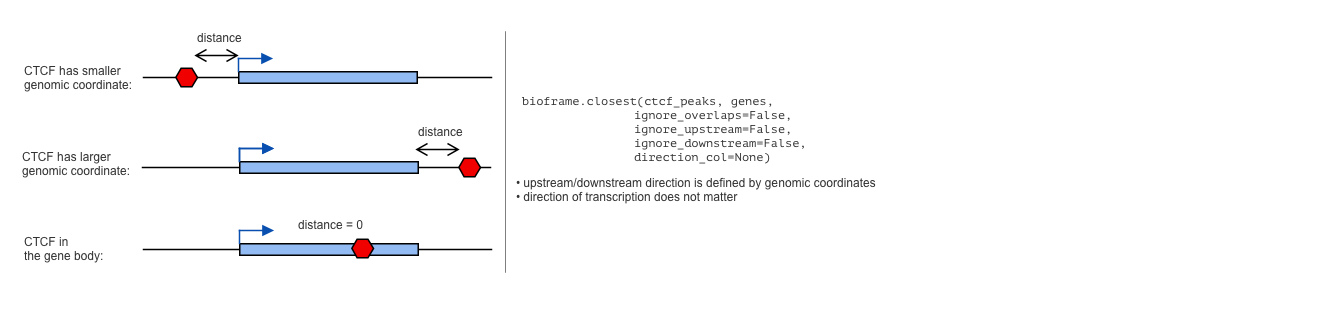
Here, we want to assign each peak (feature) to a gene (input table).

peaks_closest = bioframe.closest(genes, ctcf_peaks)

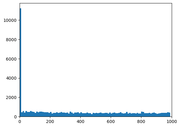
# Plot the distribution of distances from peaks to genes:
plt.hist(peaks_closest["distance"], np.arange(0, 1e3, 10))
plt.xlim([0, 1e3])

(0.0, 1000.0)

Ignore upstream/downstream peaks from genes (strand-indifferent version)

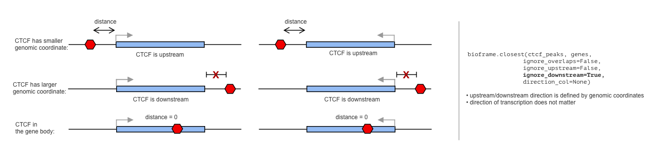
Sometimes you may want to ignore all the CTCFs upstream from the genes.

By default, bioframe.overlap does not know the orintation of the genes, and thus assumes that the upstream/downstream is defined by the genomic coordinate (upstream is the direction towards the smaller coordinate):

peaks_closest_upstream_nodir = bioframe.closest(
    genes,
    ctcf_peaks,
    ignore_overlaps=False,
    ignore_upstream=False,
    ignore_downstream=True,
    direction_col=None,
)

peaks_closest_downstream_nodir = bioframe.closest(
    genes,
    ctcf_peaks,
    ignore_overlaps=False,
    ignore_upstream=True,
    ignore_downstream=False,
    direction_col=None,
)

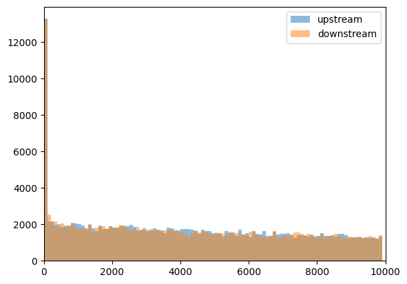
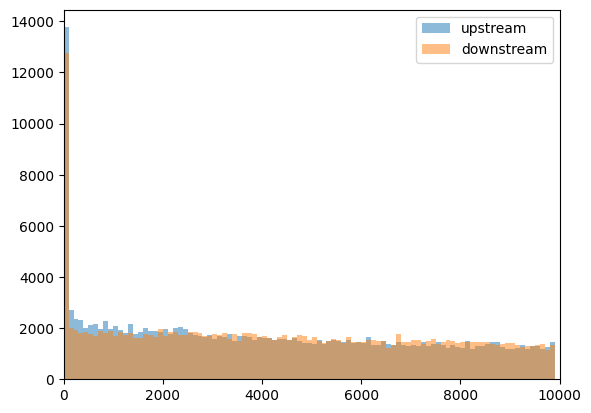
Note that distribution did not change much, and upstream and downstream distances are very similar:

plt.hist(
    peaks_closest_upstream_nodir["distance"],
    np.arange(0, 1e4, 100),
    alpha=0.5,
    label="upstream",
)
plt.hist(
    peaks_closest_downstream_nodir["distance"],
    np.arange(0, 1e4, 100),
    alpha=0.5,
    label="downstream",
)
plt.xlim([0, 1e4])
plt.legend()

<matplotlib.legend.Legend at 0x7f33a44537f0>

Ignore upstream/downstream peaks from genes (strand-aware version)

More biologically relevant approach will be to define upstream/downstream by strand of the gene. CTCF upstream of transcription start site might play different role than CTCF after transcription end site.

bioframe.closest has the parameter direction_col to control for that:

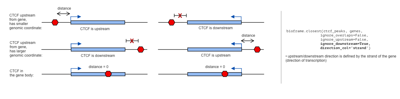
# Note that "strand" here is the column name in genes table:
peaks_closest_upstream_dir = bioframe.closest(
    genes,
    ctcf_peaks,
    ignore_overlaps=False,
    ignore_upstream=False,
    ignore_downstream=True,
    direction_col="strand",
)

peaks_closest_downstream_dir = bioframe.closest(
    genes,
    ctcf_peaks,
    ignore_overlaps=False,
    ignore_upstream=True,
    ignore_downstream=False,
    direction_col="strand",
)

plt.hist(
    peaks_closest_upstream_dir["distance"],
    np.arange(0, 1e4, 100),
    alpha=0.5,
    label="upstream",
)
plt.hist(
    peaks_closest_downstream_dir["distance"],
    np.arange(0, 1e4, 100),
    alpha=0.5,
    label="downstream",
)
plt.xlim([0, 1e4])
plt.legend()

<matplotlib.legend.Legend at 0x7f338e3e5660>

CTCF peaks upstream of the genes are more enriched at short distances to TSS, if we take the strand into account.